Sometimes the most interesting findings start with a simple question. After publishing my recent post on Oracle 26ai JOIN TO ONE, Iudith Mentzel pointed out something in one of the query transformations that looked perfectly logical – but turned out not to describe what Oracle actually does.
A small test led me one level deeper, from DBMS_UTILITY.EXPAND_SQL_TEXT to the CBO trace, and revealed another interesting aspect of JOIN TO ONE: the way Oracle handles its implicit LEFT OUTER JOIN.
In the previous post, I used DBMS_UTILITY.EXPAND_SQL_TEXT to investigate how Oracle implements the TO ONE guarantee. If Oracle cannot rely on a primary or unique key to guarantee that there is at most one matching row, the expanded SQL contains an additional correlated scalar subquery. Since a scalar subquery cannot return more than one row, this provides an elegant way to detect a violation of the TO ONE semantics.
As a reminder, Listing 1 shows the query and the transformation we see when there is no primary or unique key constraint in ENABLE VALIDATE state on PROMOTIONS.PROMO_ID.
select sum(s.amount_sold)
from   sales s
       join to one (promotions p)
where  p.promo_name like 'NO PROMOTION%';

SELECT SUM ("A1"."AMOUNT_SOLD_0")     "SUM(S.AMOUNT_SOLD)"
FROM   (SELECT "A3"."AMOUNT_SOLD"     "AMOUNT_SOLD_0",
               "A2"."PROMO_NAME"      "PROMO_NAME_1"
        FROM   "ONF"."SALES" "A3", "ONF"."PROMOTIONS" "A2"
        WHERE  "A3"."PROMO_ID" = "A2"."PROMO_ID"
        AND    'P' = (SELECT 'P'  "C"
                      FROM   "ONF"."PROMOTIONS" "A4"
                      WHERE  "A3"."PROMO_ID" = "A4"."PROMO_ID")) "A1"
WHERE  "A1"."PROMO_NAME_1" LIKE 'NO PROMOTION%';
Listing 1: JOIN TO ONE query and SQL returned by EXPAND_SQL_TEXT
At least, that was the picture we had so far.
One of the comments on the post raised a very good question: if this scalar subquery is added as a filtering predicate, wouldn’t it also eliminate rows without a match and therefore effectively turn the implicit LEFT OUTER JOIN into an INNER JOIN?
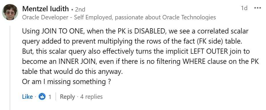
Looking at the SQL returned by EXPAND_SQL_TEXT, that conclusion makes perfect sense. But a simple test proves that Oracle does preserve the outer join semantics. So there must be more going on.
Let’s do a very simple test with two tables and without any constraints:
drop table t1 purge;
drop table t2 purge;

create table t1 (
    id  number,
    val varchar2(10)
);

create table t2 (
    id  number,
    val varchar2(10)
);

-- Two rows on the preserved side
insert into t1 values (1, 'A');
insert into t1 values (2, 'B');

-- ID 1: exactly one match
-- ID 2: no match
insert into t2 values (1, 'A');

commit;
Listing 2: Minimal test case without constraints
Now the simple LEFT JOIN query produces the expected result in Listing 3 (lines 2–8). The next query (lines 12–18) uses the new JOIN TO ONE syntax. Since we don’t have any FK-PK constraints, we need to provide the ON condition explicitly. The default join semantics for JOIN TO ONE is LEFT OUTER JOIN, so we can omit the explicit join type. Again, the result is exactly what we expect: the row with ID=2 from the preserved table T1 remains in the result, while the columns from T2 are NULL.
Next, let’s call EXPAND_SQL_TEXT to see the transformed query. As expected, we find the scalar subquery we are already familiar with (lines 53–55). Now let’s execute this transformed query. It should, of course, return the same result as the original query, right?
Wrong!
The transformed query behaves like an INNER JOIN: the row with ID=2 is filtered out.
SQL> -- Query with LEFT JOIN to T2
SQL> SELECT t1.id, t1.val, t2.val
FROM   t1 LEFT JOIN t2 ON t1.id = t2.id

        ID VAL        VAL_1
---------- ---------- ----------
         1 A          A
         2 B
2 rows selected.

SQL> -- JOIN TO ONE (default is LEFT OUTER JOIN)
SQL> SELECT t1.id, t1.val, t2.val
FROM   t1 JOIN TO ONE (t2 ON t1.id = t2.id)

        ID VAL        VAL_1
---------- ---------- ----------
         1 A          A
         2 B
2 rows selected.

SQL> -- get the transformation behind it
SQL> WITH FUNCTION get_sql (p_sql IN CLOB) RETURN CLOB IS
p_sql_out CLOB;
BEGIN
  DBMS_UTILITY.EXPAND_SQL_TEXT (p_sql, p_sql_out);
  RETURN p_sql_out;
END;
SELECT get_sql(q'[
SELECT t1.id, t1.val, t2.val
FROM   t1 JOIN TO ONE (t2 ON t1.id = t2.id)]') AS transformation

TRANSFORMATION
--------------------------------------------------------------------------------
SELECT "A1"."QCSJ_C000000000300000_0" "ID","A1"."QCSJ_C000000000300002_1" "VAL",
"A1"."QCSJ_C000000000300003_3" "VAL" FROM  (SELECT "A3"."ID" "QCSJ_C000000000300
000_0","A3"."VAL" "QCSJ_C000000000300002_1","A2"."ID" "QCSJ_C000000000300001","A
2"."VAL" "QCSJ_C000000000300003_3" FROM "SH"."T1" "A3","SH"."T2" "A2" WHERE "A3"
."ID"="A2"."ID" AND 'T2'= (SELECT 'T2' "C" FROM "SH"."T2" "A4" WHERE "A3"."ID"="
A4"."ID")) "A1"

1 row selected.

SQL> -- Execute the transformed query
SQL> SELECT "A1"."QCSJ_C000000000300000_0"     "ID",
       "A1"."QCSJ_C000000000300002_1"     "VAL",
       "A1"."QCSJ_C000000000300003_3"     "VAL"
  FROM (SELECT "A3"."ID"      "QCSJ_C000000000300000_0",
               "A3"."VAL"     "QCSJ_C000000000300002_1",
               "A2"."ID"      "QCSJ_C000000000300001",
               "A2"."VAL"     "QCSJ_C000000000300003_3"
          FROM "SH"."T1" "A3", "SH"."T2" "A2"
         WHERE     "A3"."ID" = "A2"."ID"
               AND 'T2' = (SELECT 'T2'     "C"
                             FROM "SH"."T2" "A4"
                            WHERE "A3"."ID" = "A4"."ID")) "A1"

        ID VAL        VAL_1
---------- ---------- ----------
         1 A          A
1 row selected.
Listing 3: Different results for the original query and the SQL returned by EXPAND_SQL_TEXT
So we have a contradiction: the original JOIN TO ONE query clearly preserves the outer join semantics, while the SQL returned by EXPAND_SQL_TEXT, when executed literally, does not.
Apparently, EXPAND_SQL_TEXT is not showing us the whole story. To find out what Oracle actually does with this query, we need to go one level deeper and look at the optimizer trace.
Going One Level Deeper: The CBO Trace
For this test, I used a small function I previously showed in this post about SQL macros to retrieve the final SQL from the CBO trace.
...
Final query after transformations: qb SEL$FF1EE860 (#1):
******* UNPARSED QUERY IS *******

SELECT "T1"."ID"                  "ID",
       "T1"."VAL"                 "VAL",
       "VW_LAT_CDDD7452"."ITEM_2" "VAL"
FROM   "SH"."T1" "T1",
       LATERAL (
         (SELECT "T2"."VAL" "ITEM_2"
          FROM   "SH"."T2" "T2"
          WHERE  "T1"."ID" = "T2"."ID"
          AND    (SELECT 'T2' "C"
                  FROM   "SH"."T2" "T2"
                  WHERE  "T2"."ID" = "T1"."ID") = 'T2')
       )(+) "VW_LAT_CDDD7452"

*************************
......
Listing 4: Final query after transformations from the CBO trace
And there is the missing piece. The correlated scalar subquery is still there, but it is now inside a LATERAL view. More importantly, the entire lateral view is outer-joined to T1, as indicated by the (+).
This preserves exactly the semantics we need. If there is no matching row in T2, the lateral view returns no row, but the outer join preserves the row from T1 and returns NULL for the T2 columns. With one matching row, the join behaves normally. And with more than one matching row, the scalar subquery still enforces the TO ONE guarantee.
I used to rely on DBMS_UTILITY.EXPAND_SQL_TEXT for looking at query transformations, as many others do. It is a very convenient trick and it can reveal quite a lot about how Oracle rewrites a query.
But we should also remember what EXPAND_SQL_TEXT is actually documented for: expanding references to views. Using it to inspect other query transformations is undocumented behavior. And, once again, this is a good reminder of a familiar rule when working with Oracle: you cannot rely on undocumented features.
Interestingly, within its documented purpose, the documentation also states that the resulting SQL is semantically equivalent to the input query, with a few documented caveats. Our example shows why extending that expectation to other, undocumented transformations is risky. So EXPAND_SQL_TEXT remains a useful diagnostic trick – just not the ultimate source of truth for every query transformation.
From Transformation to Execution Plan
Now that we know how Oracle preserves the LEFT OUTER JOIN semantics, let’s go back to the original JOIN TO ONE query and look at its execution plan.
Listing 5 shows the final transformed query from the CBO trace together with the execution plan of the original JOIN TO ONE query. The CBO transformation already suggests that preserving the outer join semantics requires more than the scalar-subquery check alone. Listing 5 shows how this translates into the execution plan.
SELECT "T1"."ID" "ID", "T1"."VAL" "VAL", "VW_LAT_CDDD7452"."ITEM_2" "VAL"
  FROM "SH"."T1"  "T1",
       LATERAL
           ( (SELECT "T2"."VAL"     "ITEM_2"
                FROM "SH"."T2" "T2"
               WHERE     "T1"."ID" = "T2"."ID"
                     AND (SELECT 'T2'     "C"
                            FROM "SH"."T2" "T2"
                           WHERE "T2"."ID" = "T1"."ID") = 'T2'))
           (+)
           "VW_LAT_CDDD7452";

--------------------------------------------------
| Id  | Operation             | Name            |
--------------------------------------------------
|   0 | SELECT STATEMENT      |                 |
|   1 |  MERGE JOIN OUTER     |                 |
|   2 |   TABLE ACCESS FULL   | T1              |
|   3 |   BUFFER SORT         |                 |
|   4 |    VIEW               | VW_LAT_A18161FF |
|*  5 |     FILTER            |                 |
|*  6 |      TABLE ACCESS FULL| T2              |
|*  7 |      TABLE ACCESS FULL| T2              |
--------------------------------------------------
Listing 5: CBO transformation and execution plan for implicit LEFT OUTER JOIN TO ONE
The transformation we saw in the CBO trace explains the more complicated plan. The outer-joined lateral view is clearly visible, together with the MERGE JOIN OUTER. It contains both the actual join to T2 and the correlated scalar subquery. The scalar subquery still has to detect multiple matches, while the surrounding outer-join structure has to preserve unmatched rows.
For comparison, with an explicit INNER JOIN TO ONE, the final transformed query is much simpler:
SELECT "T1"."ID" "ID", "T1"."VAL" "VAL", "T2"."VAL" "VAL"
  FROM "SH"."T1" "T1", "SH"."T2" "T2"
 WHERE     "T1"."ID" = "T2"."ID"
       AND (SELECT 'T2'     "C"
              FROM "SH"."T2" "T2"
             WHERE "T2"."ID" = "T1"."ID") = 'T2'

------------------------------------
| Id  | Operation           | Name |
------------------------------------
|   0 | SELECT STATEMENT    |      |
|*  1 |  FILTER             |      |
|*  2 |   HASH JOIN         |      |
|   3 |    TABLE ACCESS FULL| T2   |
|   4 |    TABLE ACCESS FULL| T1   |
|*  5 |   TABLE ACCESS FULL | T2   |
------------------------------------
Listing 6: CBO transformation and execution plan for explicit INNER JOIN TO ONE
Performance: The Runtime Check Has a Cost
In my previous post, I discussed the potential performance impact of the additional scalar-subquery check, but didn’t actually measure it. Also, most of my examples contained a filtering predicate on the joined table, effectively turning the implicit LEFT OUTER JOIN into an INNER JOIN and hiding another part of the picture. So let’s now look at both: the actual cost of the runtime check itself, and what changes when the implicit outer join really remains an outer join.
Let’s first look at a more conventional setup with indexes on the dimension keys in Listing 7. The primary key indexes are present, but the corresponding constraints are not in ENABLE VALIDATE state, so Oracle still has to enforce the TO ONE semantics at runtime. For this first test, I deliberately keep the indexes while preventing Oracle from relying on the corresponding constraints. This lets us isolate the cost of the runtime check when efficient index lookups are available.
SH>SET AUTOTRACE ON EXPLAIN
SH>
SH>select sum(s.amount_sold)
  2  from   sales s
  3  join   customers c
  4    on   c.cust_id = s.cust_id
  5  join   promotions p
  6    on   p.promo_id = s.promo_id;

SUM(S.AMOUNT_SOLD)
------------------
        98205831.2

Elapsed: 00:00:00.25

Execution Plan
----------------------------------------------------------
Plan hash value: 441219251

-------------------------------------------------------------------------------------------------------
| Id  | Operation              | Name         | Rows  | Bytes | Cost (%CPU)| Time     | Pstart| Pstop |
-------------------------------------------------------------------------------------------------------
|   0 | SELECT STATEMENT       |              |     1 |    23 |  3866   (1)| 00:00:01 |       |       |
|   1 |  SORT AGGREGATE        |              |     1 |    23 |            |          |       |       |
|*  2 |   HASH JOIN            |              |   918K|    20M|  3866   (1)| 00:00:01 |       |       |
|   3 |    INDEX FAST FULL SCAN| CUSTOMERS_PK | 55500 |   270K|    36   (0)| 00:00:01 |       |       |
|*  4 |    HASH JOIN           |              |   918K|    15M|  3827   (1)| 00:00:01 |       |       |
|   5 |     INDEX FULL SCAN    | PROMO_PK     |   503 |  2012 |     1   (0)| 00:00:01 |       |       |
|   6 |     PARTITION RANGE ALL|              |   918K|    12M|  3824   (1)| 00:00:01 |     1 |    15 |
|   7 |      TABLE ACCESS FULL | SALES        |   918K|    12M|  3824   (1)| 00:00:01 |     1 |    15 |
-------------------------------------------------------------------------------------------------------

SH>select sum(s.amount_sold)
  2  from   sales s
  3  join to one (INNER JOIN customers c  on c.cust_id = s.cust_id INNER JOIN promotions p  on p.promo_id = s.promo_id );

SUM(S.AMOUNT_SOLD)
------------------
        98205831.2

Elapsed: 00:00:00.42

Execution Plan
----------------------------------------------------------
Plan hash value: 410504316

--------------------------------------------------------------------------------------------------------
| Id  | Operation               | Name         | Rows  | Bytes | Cost (%CPU)| Time     | Pstart| Pstop |
--------------------------------------------------------------------------------------------------------
|   0 | SELECT STATEMENT        |              |     1 |    23 |  5484   (1)| 00:00:01 |       |       |
|   1 |  SORT AGGREGATE         |              |     1 |    23 |            |          |       |       |
|*  2 |   FILTER                |              |       |       |            |          |       |       |
|*  3 |    HASH JOIN            |              |   918K|    20M|  3871   (1)| 00:00:01 |       |       |
|   4 |     INDEX FAST FULL SCAN| CUSTOMERS_PK | 55500 |   270K|    36   (0)| 00:00:01 |       |       |
|*  5 |     HASH JOIN           |              |   918K|    15M|  3833   (1)| 00:00:01 |       |       |
|   6 |      INDEX FULL SCAN    | PROMO_PK     |   503 |  2012 |     1   (0)| 00:00:01 |       |       |
|   7 |      PARTITION RANGE ALL|              |   918K|    12M|  3830   (1)| 00:00:01 |     1 |    15 |
|   8 |       TABLE ACCESS FULL | SALES        |   918K|    12M|  3830   (1)| 00:00:01 |     1 |    15 |
|*  9 |    INDEX UNIQUE SCAN    | PROMO_PK     |     1 |     4 |     0   (0)| 00:00:01 |       |       |
|* 10 |    INDEX UNIQUE SCAN    | CUSTOMERS_PK |     1 |     5 |     1   (0)| 00:00:01 |       |       |
--------------------------------------------------------------------------------------------------------

SH>select sum(s.amount_sold)
  2  from   sales s
  3  join to one (customers c  on c.cust_id = s.cust_id, promotions p  on p.promo_id = s.promo_id );

SUM(S.AMOUNT_SOLD)
------------------
        98205831.2

Elapsed: 00:00:01.77

Execution Plan
----------------------------------------------------------
Plan hash value: 4010859135

-----------------------------------------------------------------------------------------------------------
| Id  | Operation               | Name            | Rows  | Bytes | Cost (%CPU)| Time     | Pstart| Pstop |
-----------------------------------------------------------------------------------------------------------
|   0 | SELECT STATEMENT        |                 |     1 |    14 |  1841K  (1)| 00:01:12 |       |       |
|   1 |  SORT AGGREGATE         |                 |     1 |    14 |            |          |       |       |
|   2 |   MERGE JOIN OUTER      |                 |   918K|    12M|  1841K  (1)| 00:01:12 |       |       |
|   3 |    MERGE JOIN OUTER     |                 |   918K|    12M|  1841K  (1)| 00:01:12 |       |       |
|   4 |     PARTITION RANGE ALL |                 |   918K|    12M|  3824   (1)| 00:00:01 |     1 |    15 |
|   5 |      TABLE ACCESS FULL  | SALES           |   918K|    12M|  3824   (1)| 00:00:01 |     1 |    15 |
|   6 |     BUFFER SORT         |                 |     1 |       |  1838K  (1)| 00:01:12 |       |       |
|   7 |      VIEW               | VW_LAT_A22CA6F4 |     1 |       |     2   (0)| 00:00:01 |       |       |
|*  8 |       FILTER            |                 |       |       |            |          |       |       |
|*  9 |        INDEX UNIQUE SCAN| CUSTOMERS_PK    |     1 |     5 |     1   (0)| 00:00:01 |       |       |
|* 10 |        INDEX UNIQUE SCAN| CUSTOMERS_PK    |     1 |     5 |     1   (0)| 00:00:01 |       |       |
|  11 |    BUFFER SORT          |                 |     1 |       |  1841K  (1)| 00:01:12 |       |       |
|  12 |     VIEW                | VW_LAT_A22CA6F4 |     1 |       |     0   (0)| 00:00:01 |       |       |
|* 13 |      FILTER             |                 |       |       |            |          |       |       |
|* 14 |       INDEX UNIQUE SCAN | PROMO_PK        |     1 |     4 |     0   (0)| 00:00:01 |       |       |
|* 15 |       INDEX UNIQUE SCAN | PROMO_PK        |     1 |     4 |     0   (0)| 00:00:01 |       |       |
-----------------------------------------------------------------------------------------------------------
Listing 7: Comparing regular JOIN and JOIN TO ONE with supporting indexes
The regular INNER JOIN query finishes in 0.25 seconds. Adding JOIN TO ONE with explicit INNER JOINs increases the runtime to 0.42 seconds. The basic join strategy remains the same, but the FILTER operation performs an additional INDEX UNIQUE SCAN for each of the two dimension tables to verify the TO ONE condition.
With the implicit LEFT OUTER JOIN, the difference is more pronounced. Oracle uses the lateral views we have just seen in the CBO trace, together with MERGE JOIN OUTER operations. The query takes 1.77 seconds — still perfectly manageable, but about seven times longer than the regular join.
So, with efficient index lookups available, the additional runtime checks have a measurable but still manageable cost. But indexes and constraints are not always an option.
More complex join conditions, temporal validity, joins to views, or intermediate processing structures may not allow the TO ONE guarantee to be expressed through a primary or unique key constraint at all. And whenever larger amounts of data are processed — in ETL transformations, intermediate processing steps, or large batch jobs — full table scans and hash joins without any supporting indexes can be exactly what we want.
What If There Are No Indexes?
This brings us to the other part of the experiment: what happens to the runtime checks when there are no supporting indexes?
Rather than constructing yet another test case, let’s simply use the same SH queries again, this time without indexes on CUSTOMERS and PROMOTIONS (Listing 8).
ONF>select sum(s.amount_sold)
  2  from   sales s
  3  join   customers c
  4    on   c.cust_id = s.cust_id
  5  join   promotions p
  6    on   p.promo_id = s.promo_id;

SUM(S.AMOUNT_SOLD)
------------------
        98205831.2

Elapsed: 00:00:00.10

Execution Plan
----------------------------------------------------------
Plan hash value: 2669048432

-----------------------------------------------------------------------------------
| Id  | Operation            | Name       | Rows  | Bytes | Cost (%CPU)| Time     |
-----------------------------------------------------------------------------------
|   0 | SELECT STATEMENT     |            |     1 |    23 |  1663   (1)| 00:00:01 |
|   1 |  SORT AGGREGATE      |            |     1 |    23 |            |          |
|*  2 |   HASH JOIN          |            |   918K|    20M|  1663   (1)| 00:00:01 |
|   3 |    TABLE ACCESS FULL | CUSTOMERS  | 55500 |   270K|   422   (0)| 00:00:01 |
|*  4 |    HASH JOIN         |            |   918K|    15M|  1238   (1)| 00:00:01 |
|   5 |     TABLE ACCESS FULL| PROMOTIONS |   503 |  2012 |     6   (0)| 00:00:01 |
|   6 |     TABLE ACCESS FULL| SALES      |   918K|    12M|  1230   (1)| 00:00:01 |
-----------------------------------------------------------------------------------

ONF>select sum(s.amount_sold)
  2  from   sales s
  3  join to one (INNER JOIN customers c  on c.cust_id = s.cust_id
  4               INNER JOIN promotions p  on p.promo_id = s.promo_id );

SUM(S.AMOUNT_SOLD)
------------------
        98205831.2

Elapsed: 00:29:08.80

Execution Plan
----------------------------------------------------------
Plan hash value: 298750268

------------------------------------------------------------------------------------
| Id  | Operation             | Name       | Rows  | Bytes | Cost (%CPU)| Time     |
------------------------------------------------------------------------------------
|   0 | SELECT STATEMENT      |            |     1 |    23 |  2060K  (1)| 00:01:21 |
|   1 |  SORT AGGREGATE       |            |     1 |    23 |            |          |
|*  2 |   FILTER              |            |       |       |            |          |
|*  3 |    HASH JOIN          |            |   918K|    20M|  1668   (2)| 00:00:01 |
|   4 |     TABLE ACCESS FULL | CUSTOMERS  | 55500 |   270K|   422   (0)| 00:00:01 |
|*  5 |     HASH JOIN         |            |   918K|    15M|  1243   (2)| 00:00:01 |
|   6 |      TABLE ACCESS FULL| PROMOTIONS |   503 |  2012 |     6   (0)| 00:00:01 |
|   7 |      TABLE ACCESS FULL| SALES      |   918K|    12M|  1235   (1)| 00:00:01 |
|*  8 |    TABLE ACCESS FULL  | PROMOTIONS |     1 |     4 |     6   (0)| 00:00:01 |
|*  9 |    TABLE ACCESS FULL  | CUSTOMERS  |     1 |     5 |   423   (1)| 00:00:01 |
------------------------------------------------------------------------------------

ONF>select sum(s.amount_sold)
  2  from   sales s
  3  join to one (customers c  on c.cust_id = s.cust_id
  4             , promotions p  on p.promo_id = s.promo_id );

SUM(S.AMOUNT_SOLD)
------------------
        98205831.2

Elapsed: 01:02:26.11

Execution Plan
----------------------------------------------------------
Plan hash value: 3695551726

-------------------------------------------------------------------------------------------
| Id  | Operation               | Name            | Rows  | Bytes | Cost (%CPU)| Time     |
-------------------------------------------------------------------------------------------
|   0 | SELECT STATEMENT        |                 |     1 |    14 |   787M  (1)| 08:32:42 |
|   1 |  SORT AGGREGATE         |                 |     1 |    14 |            |          |
|   2 |   MERGE JOIN OUTER      |                 |   918K|    12M|   787M  (1)| 08:32:42 |
|   3 |    MERGE JOIN OUTER     |                 |   918K|    12M|   776M  (1)| 08:25:31 |
|   4 |     TABLE ACCESS FULL   | SALES           |   918K|    12M|  1230   (1)| 00:00:01 |
|   5 |     BUFFER SORT         |                 |     1 |       |   776M  (1)| 08:25:31 |
|   6 |      VIEW               | VW_LAT_A22CA6F4 |     1 |       |   845   (1)| 00:00:01 |
|*  7 |       FILTER            |                 |       |       |            |          |
|*  8 |        TABLE ACCESS FULL| CUSTOMERS       |     1 |     5 |   423   (1)| 00:00:01 |
|*  9 |        TABLE ACCESS FULL| CUSTOMERS       |     1 |     5 |   423   (1)| 00:00:01 |
|  10 |    BUFFER SORT          |                 |     1 |       |   787M  (1)| 08:32:42 |
|  11 |     VIEW                | VW_LAT_A22CA6F4 |     1 |       |    12   (0)| 00:00:01 |
|* 12 |      FILTER             |                 |       |       |            |          |
|* 13 |       TABLE ACCESS FULL | PROMOTIONS      |     1 |     4 |     6   (0)| 00:00:01 |
|* 14 |       TABLE ACCESS FULL | PROMOTIONS      |     1 |     4 |     6   (0)| 00:00:01 |
-------------------------------------------------------------------------------------------
Listing 8: Comparing regular JOIN and JOIN TO ONE without supporting indexes
| Query | With indexes | Without indexes |
|---|---|---|
| Regular INNER JOIN | 0.25 s | 0.10 s |
| INNER JOIN TO ONE | 0.42 s | 29 min 09 s |
| LEFT OUTER JOIN TO ONE | 1.77 s | 1 h 02 min |
The regular join is actually faster in this setup and finishes in just 0.10 seconds. Oracle full-scans the three tables and combines them using two hash joins.
With explicit INNER JOIN TO ONE, however, the runtime jumps to 29 minutes. The two hash joins are still there, but so are the correlated runtime checks. Without indexes, the correlated checks repeatedly access the corresponding dimension tables using full table scans.
And with the implicit LEFT OUTER JOIN, things get even worse: the query takes more than an hour. The lateral-view transformation now combines the outer joins with repeated full scans of the dimension tables.
So this is where I would be particularly careful with JOIN TO ONE: large-volume processing on tables that deliberately have no supporting indexes or validated uniqueness constraints. A regular full-scan/hash-join plan can be extremely efficient in such a scenario, while the current implementation of the TO ONE runtime checks can completely change the performance characteristics of the query.
Of course, missing or disabled constraints are not the only reason why Oracle may have to perform the runtime check. There are also joins for which uniqueness simply cannot be expressed by a primary or unique key constraint — for example, more complex join conditions, joins involving temporal validity, or joins to views. And there are valid processing scenarios where supporting indexes are deliberately avoided and uniqueness is not enforced through constraints.
In all these cases, the runtime enforcement of TO ONE is actually one of the attractive aspects of the feature. Unfortunately, with the current implementation, it is exactly these cases where the additional check can become expensive.
Final thoughts
These tests add an important performance perspective to the conclusions from my previous post, particularly for data warehouse workloads. With its current implementation, for queries processing larger amounts of data, I would use it only where the TO ONE semantics are already guaranteed by an ENABLE VALIDATE primary or unique key constraint and no additional runtime check is required.
This may look quite different in OLTP or application development. There, joins often involve only a small number of rows, and properly defined and enabled constraints are often part of the application data model anyway. Even where a runtime check is required, its cost may be negligible — and if it isn’t, that might actually be a good reason to revisit the data model.
I still very much like the concept behind JOIN TO ONE, particularly the ability to detect accidental row multiplication where constraints cannot provide that guarantee. Unfortunately, these are precisely the cases where the current implementation makes me reluctant to use it for large-volume processing.
But this is still a very young feature. I hope Oracle is already working on making the runtime enforcement more efficient. If that part can be improved, my conclusion could look quite different.
Hello Andrej,
It is not exactly clear to me why the execution plan shows a MERGE JOIN OUTER, because the LATERAL inline view already filters using the correlated column from the T1 table, so conceptually this looks more like a NESTED LOOPS OUTER.
The duplicate filter with the same (join) condition against each of the dimension tables looks to me a little like an “overkill”, if its entire purpose is just to avoid multiplying the T1 rows.
Speaking in “basic steps”, i am not sure that, as an alternative solution to using the scalar check query “row by row”, it wouldn’t be better to perform all the outer joins as usual and then, with the final result set available, apply some analytic function(s) on top of this result set to validate that each row from the left side (here T1) table was not multiplied, something along the lines of
SELECT COUNT(*) OVER( PARTITION BY result_key) cnt_per_key
FROM (
SELECT T1.ID as result_key, …
FROM …
) join_result_set
QUALIFY ( cnt_per_key > 1 )
and, if this query DOES return any rows, then raise the “multiple rows” violation error …
I just wonder how does JOIN TO ONE work in case that the FK side
is not just a single table, like here T1, but some other result set,
like a VIEW or a join of several tables, aka, in case that we do not have a single column ( like here T1.ID or possibly T1.ROWID ) on which to base the “row multiplication” avoiding logic.
The concept of a “row” for the left “table” in such a case could be more tricky, if JOIN TO ONE works at all in such a case.
Just a few fast thoughts, after an EXCELLENT post from you, as ALWAYS :):)
I am pretty sure that continuation(s) will follow 🙂
Thanks Iudith!
I think such an approach is certainly worth considering and, for the examples I tested here, I’m quite sure it would be much more efficient.
However, I don’t think this is something that could simply be implemented as another query transformation. The database would need a way to perform the join and validate the TO ONE semantics as part of the execution itself. This is actually what I had in mind in my first post when I speculated about a dedicated new operation for JOIN TO ONE. In other words, rather than expressing the check through additional SQL constructs, I would love to see the execution engine understand TO ONE natively.
And I think you have already identified one of the challenges of this approach yourself. 🙂 JOIN TO ONE itself doesn’t need to know what uniquely identifies a row on the left side — it can just use the values from the join condition. But for a validation after the join, we would need exactly such an identity to detect which result rows came from the same left-side row. With a more complex result set, that may indeed become tricky.